library(tidyverse)
library(gt)
set.seed(7)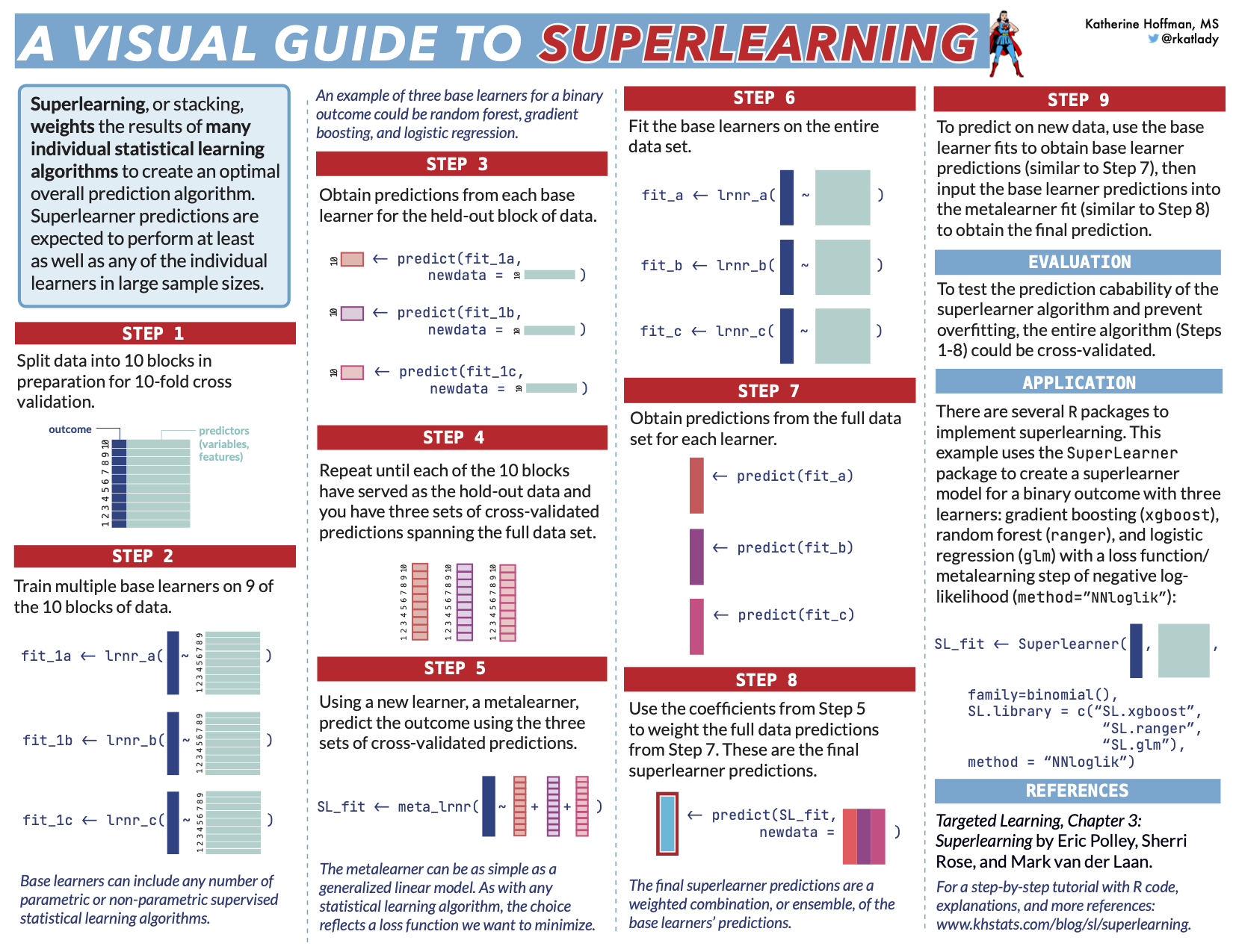
Supercuts of superlearning
- Superlearning is a technique for prediction that involves combining many individual statistical algorithms (commonly called “data-adaptive” or “machine learning” algorithms) to create a new, single prediction algorithm that is expected to perform at least as well as any of the individual algorithms.
- The superlearner algorithm “decides” how to combine, or weight, the individual algorithms based upon how well each one minimizes a specified loss function, for example, the mean squared error (MSE). This is done using cross-validation to avoid overfitting.
- The motivation for this type of “ensembling” is that a mix of multiple algorithms may be more optimal for a given data set than any single algorithm. For example, a tree based model averaged with a linear model (e.g. random forests and LASSO) could smooth some of the model’s edges to improve predictive performance.
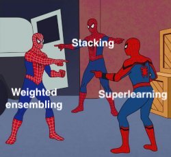
- Superlearning is also called stacking, stacked generalizations, and weighted ensembling by different specializations within the realms of statistics and data science.
Superlearning, step by step
First I’ll go through the algorithm one step at a time using a simulated data set.
Initial set-up: Load libraries, set seed, simulate data
For simplicity I’ll show the concept of superlearning using only four variables (AKA features or predictors) to predict a continuous outcome. Let’s first simulate a continuous outcome, y, and four potential predictors, x1, x2, x3, and x4.
n <- 5000
obs <- tibble(
  id = 1:n,
  x1 = rnorm(n),
  x2 = rbinom(n, 1, plogis(10*x1)),
  x3 = rbinom(n, 1, plogis(x1*x2 + .5*x2)),
  x4 = rnorm(n, mean=x1*x2, sd=.5*x3),
  y = x1 + x2 + x2*x3 + sin(x4)
)
gt(head(obs)) %>%
  tab_header("Simulated data set") %>%
fmt_number(everything(),decimals=3)| Simulated data set | |||||
| id | x1 | x2 | x3 | x4 | y |
|---|---|---|---|---|---|
| 1.000 | 2.287 | 1.000 | 1.000 | 1.385 | 5.270 |
| 2.000 | −1.197 | 0.000 | 0.000 | 0.000 | −1.197 |
| 3.000 | −0.694 | 0.000 | 0.000 | 0.000 | −0.694 |
| 4.000 | −0.412 | 0.000 | 1.000 | −0.541 | −0.928 |
| 5.000 | −0.971 | 0.000 | 0.000 | 0.000 | −0.971 |
| 6.000 | −0.947 | 0.000 | 1.000 | −0.160 | −1.107 |
Step 1: Split data into K folds
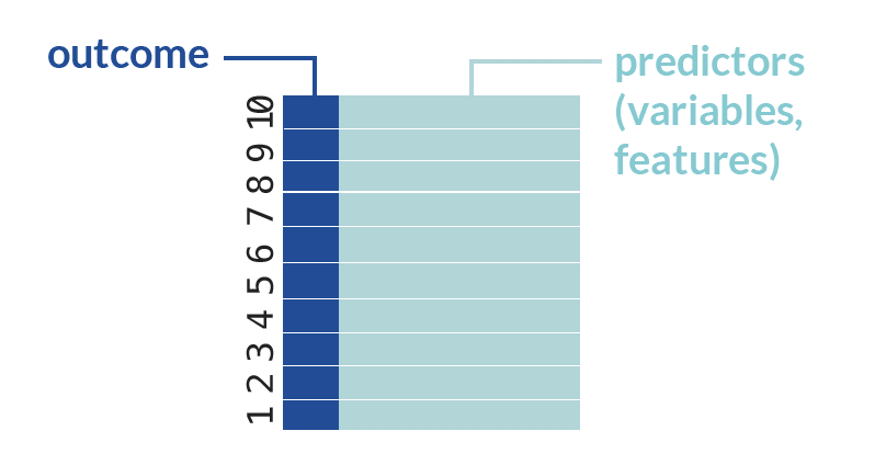 The superlearner algorithm relies on K-fold cross-validation (CV) to avoid overfitting. We will start this process by splitting the data into 10 folds. The easiest way to do this is by creating indices for each CV fold.
k <- 10 # 10 fold cv
cv_index <- sample(rep(1:k, each = n/k)) # create indices for each CV fold. We need each fold K to contain n (all the rows of our data set) divided by k rows. in our example this is 5000/10 = 500 rows in each fold
Step 2: Fit base learners for first CV-fold
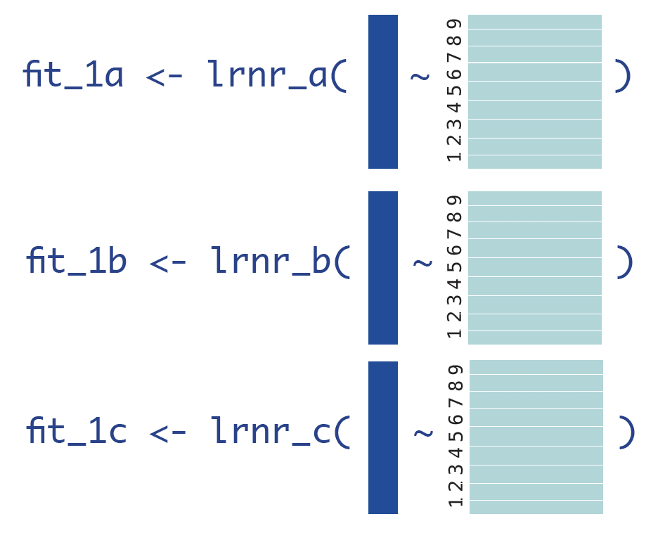
Recall that in K-fold CV, each fold serves as the validation set one time. In this first round of CV, we will train all of our base learners on all the CV folds (k = 1,2,…,9) except for the very last one: cv_index == 10.
The individual algorithms or base learners that we’ll use here are three linear regressions with differently specified parameters:
Learner A: \(Y=\beta_0 + \beta_1 X_2 + \beta_2 X_4 + \epsilon\)
Learner B: \(Y=\beta_0 + \beta_1 X_1 + \beta_2 X_2 + \beta_3 X_1 X_3 + \beta_4 sin(X_4) + \epsilon\)
Learner C: \(Y=\beta_0 + \beta_1 X_1 + \beta_2 X_2 + \beta_3 X_3 + \beta_4 X_1 X_2 + \beta_5 X_1 X_3 + \beta_6 X_2 X_3 + \beta_7 X_1 X_2 X_3 + \epsilon\)
cv_train_1 <- obs[-which(cv_index == 10),] # make a data set that contains all observations except those in k=1
fit_1a <- glm(y ~ x2 + x4, data=cv_train_1) # fit the first linear regression on that training data
fit_1b <- glm(y ~ x1 + x2 + x1*x3 + sin(x4), data=cv_train_1) # second LR fit on the training data
fit_1c <- glm(y ~ x1*x2*x3, data=cv_train_1) # and the third LR
I am only using the linear regressions so that code for running more complicated regressions does not take away from understanding the general superlearning algorithm.
Superlearning actually works best if you use a diverse set, or superlearner library, of base learners. For example, instead of three linear regressions, we could use a least absolute shrinkage estimator (LASSO), random forest, and multivariate adaptive splines (MARS). Any parametric or non-parametric supervised machine learning algorithm can be included as a base learner.
Step 3: Obtain predictions for first CV-fold
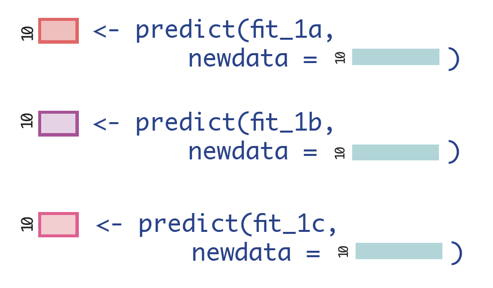
We can then get use our validation data, cv_index == 10, to obtain our first set of cross-validated predictions.
cv_valid_1 <- obs[which(cv_index == 10),] # make a data set that only contains observations except in k=10
pred_1a <- predict(fit_1a, newdata = cv_valid_1) # use that data set as the validation for all the models in the SL library
pred_1b <- predict(fit_1b, newdata = cv_valid_1)
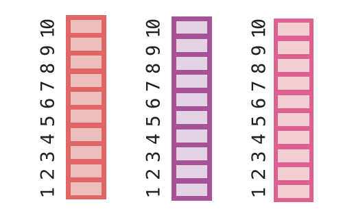
pred_1c <- predict(fit_1c, newdata = cv_valid_1)Since we have 5000 observations, that gives us three vectors of length 500: a set of predictions for each of our Learners A, B, and C.
length(pred_1a) # double check we only have n/k predictions ...we do :-)[1] 500head(cbind(pred_1a, pred_1b, pred_1c)) %>%
as.data.frame() %>% gt() %>%
fmt_number(everything(), decimals = 2) %>%
tab_header("First CV round of predictions") | First CV round of predictions | ||
| pred_1a | pred_1b | pred_1c |
|---|---|---|
| −0.77 | −0.81 | −0.69 |
| 2.54 | 1.89 | 1.63 |
| 0.19 | 0.60 | −0.32 |
| 2.46 | 2.69 | 2.98 |
| 3.63 | 4.04 | 3.73 |
| 3.59 | 3.23 | 3.15 |
Step 4: Obtain CV predictions for entire data set
We’ll want to get those predictions for every fold. So, using your favorite for loop, apply statement, or mapping function, fit the base learners and obtain predictions for each of them, so that there are 1000 predictions – one for every point in observations.
The way I chose to code this was to make a generic function that combines Step 2 (base learners fit to the training data) and Step 3 (predictions on the validation data), then use map_dfr() from the purrr package to repeat over all 10 CV folds. I saved the results in a new data frame called cv_preds.
cv_folds <- as.list(1:k)
names(cv_folds) <- paste0("fold",1:k)

get_preds <- function(fold){   # function that does the same procedure as step 2 and 3 for any CV fold
  cv_train <- obs[-which(cv_index == fold),]  # make a training data set that contains all data except fold k
  fit_a <- glm(y ~ x2 + x4, data=cv_train)  # fit all the base learners to that data
  fit_b <- glm(y ~ x1 + x2 + x1*x3 + sin(x4), data=cv_train)
  fit_c <- glm(y ~ x1*x2*x3, data=cv_train)
  cv_valid <- obs[which(cv_index == fold),]  # make a validation data set that only contains data from fold k
  pred_a <- predict(fit_a, newdata = cv_valid)  # obtain predictions from all the base learners for that validation data
  pred_b <- predict(fit_b, newdata = cv_valid)
  pred_c <- predict(fit_c, newdata = cv_valid)
  return(data.frame("obs_id" = cv_valid$id, "cv_fold" = fold, pred_a, pred_b, pred_c))  # save the predictions and the ids of the observations in a data frame
}

cv_preds <- purrr::map_dfr(cv_folds, ~get_preds(fold = .x)) # map_dfr loops through every fold (1:k) and binds the rows of the listed results together

cv_preds %>% arrange(obs_id) %>% head() %>% as.data.frame() %>% gt() %>%
  fmt_number(cv_fold:pred_c, decimals=2) %>%
tab_header("All CV predictions for all three base learners") | All CV predictions for all three base learners | ||||
| obs_id | cv_fold | pred_a | pred_b | pred_c |
|---|---|---|---|---|
| 1 | 7.00 | 3.74 | 5.42 | 5.28 |
| 2 | 6.00 | −0.77 | −1.19 | −1.20 |
| 3 | 10.00 | −0.77 | −0.81 | −0.69 |
| 4 | 8.00 | −1.39 | −0.77 | −0.41 |
| 5 | 2.00 | −0.78 | −1.02 | −0.97 |
| 6 | 9.00 | −0.96 | −1.04 | −0.94 |
Step 5: Choose and compute loss function of interest via metalearner
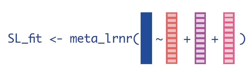
This is the key step of the superlearner algorithm: we will use a new learner, a metalearner, to take information from all of the base learners and create that new algorithm.
Now that we have cross-validated predictions for every observation in the data set, we want to merge those CV predictions back into our main data set…
obs_preds <-
  full_join(obs, cv_preds, by=c("id" = "obs_id"))
…so that we can minimize a final loss function of interest between the true outcome and each CV prediction. This is how we’re going to optimize our overall prediction algorithm: we want to make sure we’re “losing the least” in the way we combine our base learners’ predictions to ultimately make final predictions. We can do this efficiently by choosing a new learner, a metalearner, which reflects the final loss function of interest.
For simplicity, we’ll use another linear regression as our metalearner. Using a linear regression as a metalearner will minimize the Cross-Validated Mean Squared Error (CV-MSE) when combining the base learner predictions. Note that we could use a variety of parametric or non-parametric regressions to minimize the CV-MSE.
No matter what metalearner we choose, the predictors will always be the cross-validated predictions from each base learner, and the outcome will always be the true outcome, y.
sl_fit <- glm(y ~ pred_a + pred_b + pred_c, data = obs_preds)
broom::tidy(sl_fit) %>% gt() %>%
  fmt_number(estimate:p.value, decimals=2) %>%
tab_header("Metalearner regression coefficients") | Metalearner regression coefficients | ||||
| term | estimate | std.error | statistic | p.value |
|---|---|---|---|---|
| (Intercept) | 0.00 | 0.00 | −1.42 | 0.16 |
| pred_a | −0.02 | 0.00 | −4.75 | 0.00 |
| pred_b | 0.85 | 0.01 | 128.15 | 0.00 |
| pred_c | 0.17 | 0.01 | 30.07 | 0.00 |
This metalearner provides us with the coefficients, or weights, to apply to each of the base learners. In other words, if we have a set of predictions from Learner A, B, and C, we can obtain our best possible predictions by starting with an intercept of -0.003, then adding -0.017 \(\times\) predictions from Learner A, 0.854 \(\times\) predictions from Learner B, and 0.165 \(\times\) predictions from Learner C.
For more information on the metalearning step, check out the Appendix.
Step 6: Fit base learners on entire data set
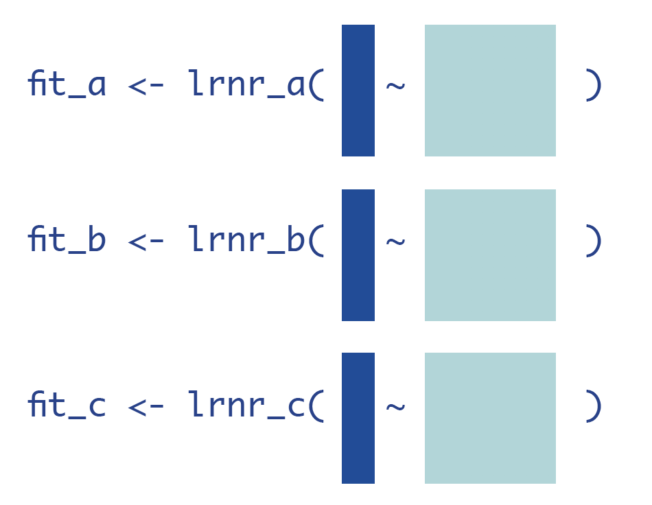
After we fit the metalearner, we officially have our superlearner algorithm, so it’s time to input data and obtain predictions! To implement the algorithm and obtain final predictions, we first need to fit the base learners on the full data set.
fit_a <- glm(y ~ x2 + x4, data=obs)
fit_b <- glm(y ~ x1 + x2 + x1*x3 + sin(x4), data=obs)
fit_c <- glm(y ~ x1*x2*x3, data=obs)
Step 7: Obtain predictions from each base learner on entire data set
We’ll use those base learner fits to get predictions from each of the base learners for the entire data set, and then we will plug those predictions into the metalearner fit. Remember, we were previously using cross-validated predictions, rather than fitting the base learners on the whole data set. This was to avoid overfitting.
pred_a <- predict(fit_a)
pred_b <- predict(fit_b)
pred_c <- predict(fit_c)
full_data_preds <- tibble(pred_a, pred_b, pred_c)
Step 8: Use metalearner fit to weight base learners
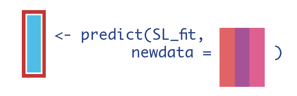
Once we have the predictions from the full data set, we can input them to the metalearner, where the output will be a final prediction for y.
sl_predictions <- predict(sl_fit, newdata = full_data_preds)
data.frame(sl_predictions = head(sl_predictions)) %>%
  gt() %>% fmt_number(sl_predictions, decimals=2) %>%
tab_header("Final SL predictions (manual)") | Final SL predictions (manual) |
| sl_predictions |
|---|
| 5.44 |
| −1.20 |
| −0.79 |
| −0.71 |
| −1.02 |
| −1.03 |
And… that’s it! Those are our superlearner predictions for the full data set.
Step 9: Obtain predictions on new data
We can now modify Step 7 and Step 8 to accommodate any new observation(s):
To predict on new data:
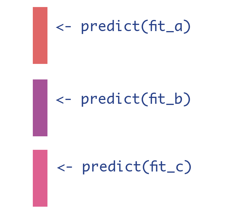
1. Use the fits from each base learner to obtain base learner predictions for the new observation(s).
2. Plug those base learner predictions into the metalearner fit.
We can generate a single new_observation to see how this would work in practice.
new_obs <- tibble(x1 = .5, x2 = 0, x3 = 0, x4 = -3)
new_pred_a <- predict(fit_a, new_obs)
new_pred_b <- predict(fit_b, new_obs)
new_pred_c <- predict(fit_c, new_obs)
new_pred_df <- tibble("pred_a" = new_pred_a, "pred_b" = new_pred_b, "pred_c" = new_pred_c)
predict(sl_fit, newdata = new_pred_df)
1
0.1183103 Our superlearner model predicts that an observation with predictors \(X_1=.5\), \(X_2=0\), \(X_3=0\), and \(X_4=-3\) will have an outcome of \(Y=0.118\).
Step 10 and beyond…
We could compute the MSE of the ensemble superlearner predictions.
sl_mse <- mean((obs$y - sl_predictions)^2)
sl_mse
[1] 0.01927392We could also add more algorithms to our base learner library (we definitely should, since we only used linear regressions!), and we could write functions to tune these algorithms’ hyperparameters over various grids. For example, if we were to include random forest in our library, we may want to tune over a number of trees and maximum bucket sizes.
We can then cross-validate this entire process to evaluate the predictive performance of our superlearner algorithm. Alternatively, we could leave a hold-out training data set to evaluate the performance.
Using the SuperLearner package
Or… we could use a package and avoid all the hand-coding. Here is how you would build an ensemble superlearner for our data with the base learner libraries of ranger (random forests), glmnet (LASSO, by default), and earth (MARS) using the SuperLearner package in R:
library(SuperLearner)
x_df <- obs %>% select(x1:x4) %>% as.data.frame()
sl_fit <- SuperLearner(Y = obs$y, X = x_df, family = gaussian(),
                     SL.library = c("SL.ranger", "SL.glmnet", "SL.earth"))
You can specify the metalearner with the method argument. The default is Non-Negative Least Squares (NNLS).
CV-Risk and Coefficient Weights
We can examine the cross-validated Risk (loss function), and the Coefficient (weight) given to each of the models.
sl_fit
Call:
SuperLearner(Y = obs$y, X = x_df, family = gaussian(), SL.library = c("SL.ranger",
    "SL.glmnet", "SL.earth"))

                     Risk      Coef
SL.ranger_All 0.013672503 0.1606329
SL.glmnet_All 0.097257031 0.0000000
SL.earth_All  0.003181357 0.8393671
From this summary we can see that the CV-risk (the default risk is MSE) in this library of base learners is smallest for SL.Earth. This translates to the largest coefficient, or weight, given to the predictions from earth.
The LASSO model implemented by glmnet has the largest CV-risk, and after the metalearning step, those predictions receive a coefficient, or weight, of 0. This means that the predictions from LASSO will not be incorporated into the final predictions at all.
Obtaining the predictions
We can extract the predictions easily via the SL.predict element of the SuperLearner fit object.
head(data.frame(sl_predictions = sl_fit$SL.predict)) %>% gt() %>%
fmt_number(everything(),decimals=2) %>% tab_header("Final SL predictions (package)") | Final SL predictions (package) |
| sl_predictions |
|---|
| 5.28 |
| −1.19 |
| −0.68 |
| −0.87 |
| −0.97 |
| −1.08 |
Cross-validated Superlearner
Recall that we can cross-validate the entire model fitting process to evaluate the predictive performance of our superlearner algorithm. This is easy with the function CV.SuperLearner(). Beware, this gets computationally burdensome very quickly!
cv_sl_fit <- CV.SuperLearner(Y = obs$y, X = x_df, family = gaussian(),
                     SL.library = c("SL.ranger", "SL.glmnet", "SL.earth"))
For more information on the SuperLearner package, take a look at this vignette.
Alternative packages to superlearn
Other packages freely available in R that can be used to implement the superlearner algorithm include sl3 (an update to the original Superlearner package), h2o, and caretEnsemble. I previously wrote a brief demo on using sl3 for an NYC R-Ladies demo.
The authors of tidymodels – a suite of packages for machine learning including recipes, parsnip, and rsample – recently came out with a new package to perform superlearning/stacking called stacks. Prior to this, Alex Hayes wrote a blog post on using tidymodels infrastructure to implement superlearning.
Coming soon… when prediction is not the end goal
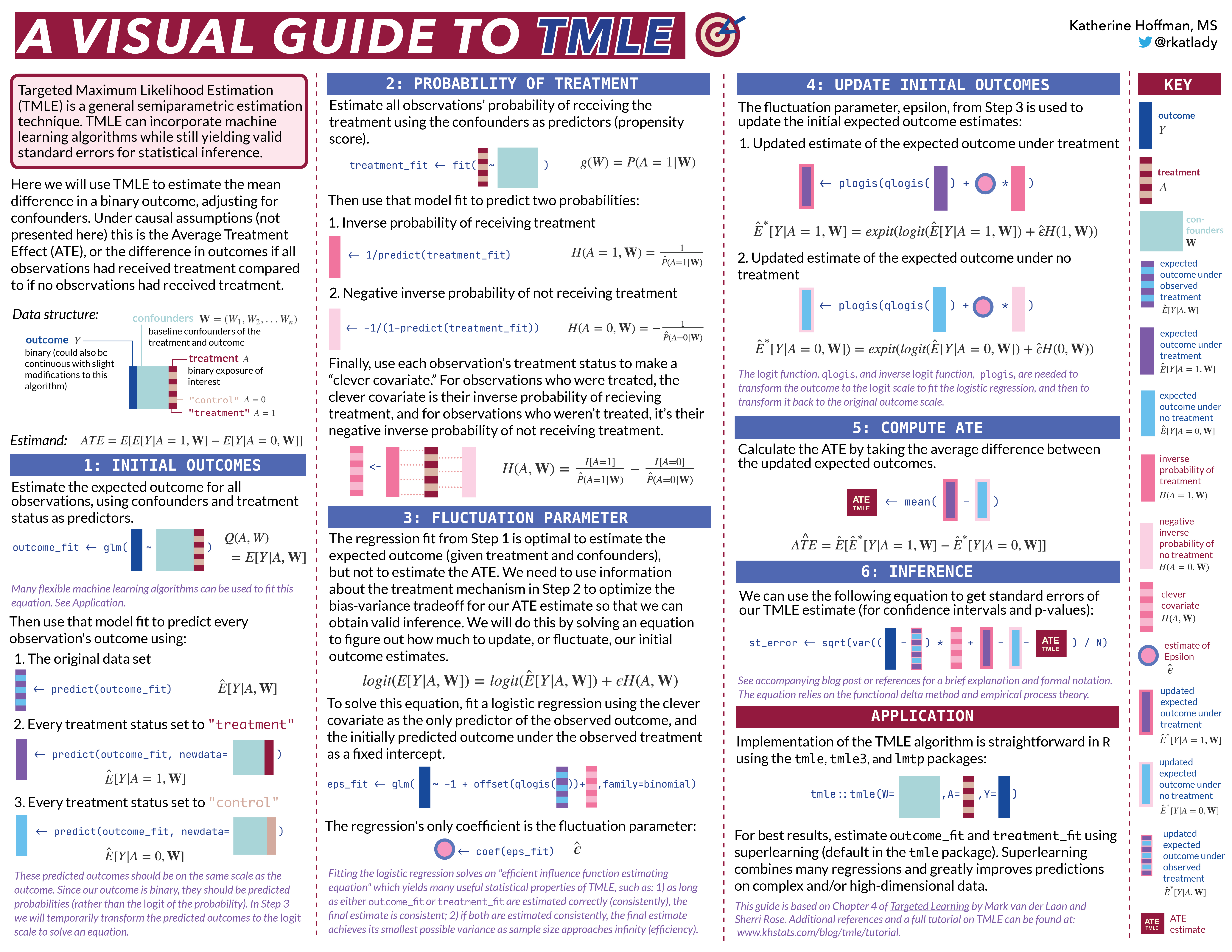
When prediction is not the end goal, superlearning combines well with semi-parametric estimation methods for statistical inference. This is the reason I was reading Targeted Learning in the first place; I am a statistician with collaborators who typically want estimates of treatment effects with confidence intervals, not predictions!
I’m working on a similar visual guide for one such semiparametric estimation method: Targeted Maximum Likelihood Estimation (TMLE)). TMLE allows the use of flexible statistical models like the superlearner algorithm when estimating treatment effects. If you found this superlearning tutorial helpful, you may be interested in this similarly visual tutorial on TMLE.
Appendix
These sections contain a bit of extra information on the superlearning algorithm, such as: intuition on manually computing the loss function of interest, explanation of the discrete superlearner, brief advice on choosing a metalearner, and a different summary visual provided in the Targeted Learning book.
Manually computing the MSE
Let’s say we have chosen our loss function of interest to be the Mean Squared Error (MSE). We could first compute the squared error \((y - \hat{y})^2\) for each CV prediction A, B, and C.
cv_sq_error <-
  obs_preds %>%
  mutate(cv_sqrd_error_a = (y-pred_a)^2,   # compute squared error for each observation
         cv_sqrd_error_b = (y-pred_b)^2,
         cv_sqrd_error_c = (y-pred_c)^2)
cv_sq_error %>%
pivot_longer(c(cv_sqrd_error_a, cv_sqrd_error_b, cv_sqrd_error_c), # make the CV squared errors long form for plotting
names_to = "base_learner",
values_to = "squared_error") %>%
mutate(base_learner = toupper(str_remove(base_learner, "cv_sqrd_error_"))) %>%
ggplot(aes(base_learner, squared_error, col=base_learner)) + # make box plots
geom_boxplot() +
theme_bw() +
guides(col=F) +
labs(x = "Base Learner", y="Squared Error", title="Squared Errors of Learner A, B, and C")Warning: The `<scale>` argument of `guides()` cannot be `FALSE`. Use "none" instead as
of ggplot2 3.3.4.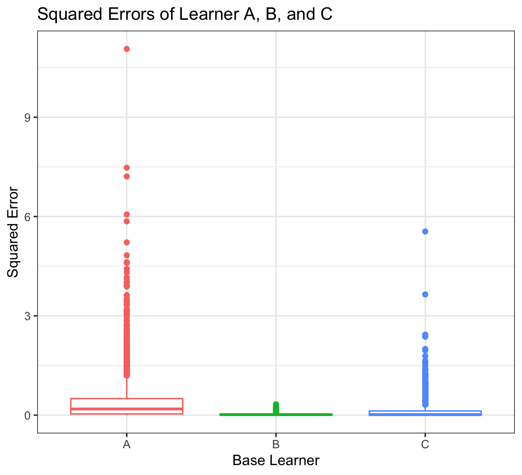
And then take the mean of those three cross-validated squared error columns, grouped by cv_fold, to get the CV-MSE for each fold.
cv_risks <-
  cv_sq_error %>%
  group_by(cv_fold) %>%
  summarise(cv_mse_a = mean(cv_sqrd_error_a),
            cv_mse_b = mean(cv_sqrd_error_b),
            cv_mse_c = mean(cv_sqrd_error_c)
            )
cv_risks %>%
  pivot_longer(cv_mse_a:cv_mse_c,
               names_to = "base_learner",
               values_to = "mse") %>%
  mutate(base_learner = toupper(str_remove(base_learner,"cv_mse_")))  %>%
  ggplot(aes(cv_fold, mse, col=base_learner)) +
  geom_point() +
  theme_bw()  +
    scale_x_continuous(breaks = 1:10) +
  labs(x = "Cross-Validation (CV) Fold", y="Mean Squared Error (MSE)", col = "Base Learner", title="CV-MSEs for Base Learners A, B, and C")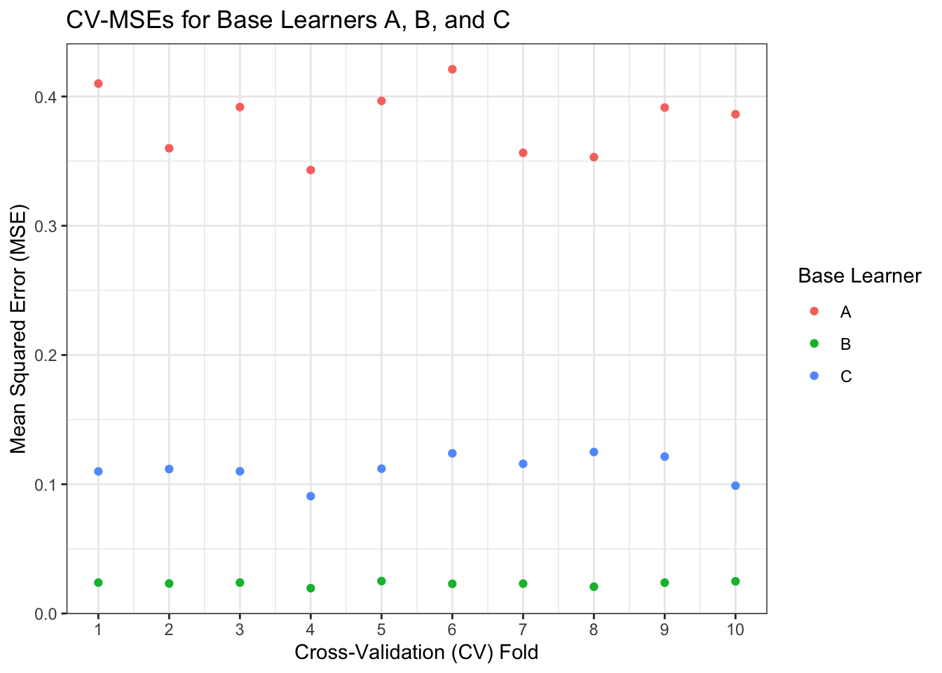
We see that across each fold, Learner B consistently has an MSE around 0.02, while Learner C hovers around 0.1, and Learner A varies between 0.35 and 0.45. We can take another mean to get the overall CV-MSE for each learner.
cv_risks %>%
  select(-cv_fold) %>%
  summarise_all(mean) %>%
  gt() %>%
fmt_number(everything(), decimals=2) %>% tab_header("CV-MSE for each base learner")| CV-MSE for each base learner | ||
| cv_mse_a | cv_mse_b | cv_mse_c |
|---|---|---|
| 0.38 | 0.02 | 0.11 |
The base learner that performs the best using our chosen loss function of interest is clearly Learner B. We can see from our data simulation code why this is true – Learner B is almost exactly the mimicking the data generating mechanism of y.
Our results align with the linear regression fit from our metalearning step; Learner B predictions received a much larger coefficient relative to Learners A and C.
Discrete Superlearner
We could stop after minimizing our loss function (MSE) and fit Learner B to our full data set, and that would be called using the discrete superlearner.
discrete_sl_predictions <- predict(glm(y ~ x1 + x2 + x1*x3 + sin(x4), data=obs))However, we can almost always create an even better prediction algorithm if we use information from all of the algorithms’ CV predictions.
Choosing a metalearner
In the Reference papers on superlearning, the metalearner which yields the best results theoretically and in practice is a convex combination optimization of learners. This means fitting the following regression, where \(\alpha_1\), \(\alpha_2\), and \(\alpha_3\) are all non-negative and sum to 1.
\(\mathrm{E}[Y|\hat{Y}_{LrnrA},\hat{Y}_{LrnrB},\hat{Y}_{LrnrC}] = \alpha_1\hat{Y}_{LrnrA} + \alpha_2\hat{Y}_{LrnrB} + \alpha_3\hat{Y}_{LrnrC}\)
The default in the Superlearner package is to fit a non-negative least squares (NNLS) regression. NNLS fits the above equation where the \(\alpha\)’s must be greater than or equal to 0 but do not necessarily sum to 1. The package then reweights the \(\alpha\)’s to force them to sum to 1. This makes the weights a convex combination, but may not yield the same optimal results as an initial convex combination optimization.
The metalearner should change with the goals of the prediction algorithm and the loss function of interest. In these examples it is the MSE, but if the goal is to build a prediction algorithm that is best for binary classification, the loss function of interest may be the rank loss, or \(1-AUC\). It is outside the scope of this post, but for more information, I recommend this paper by Erin Ledell on maximizing the Area Under the Curve (AUC) with superlearner algorithms.
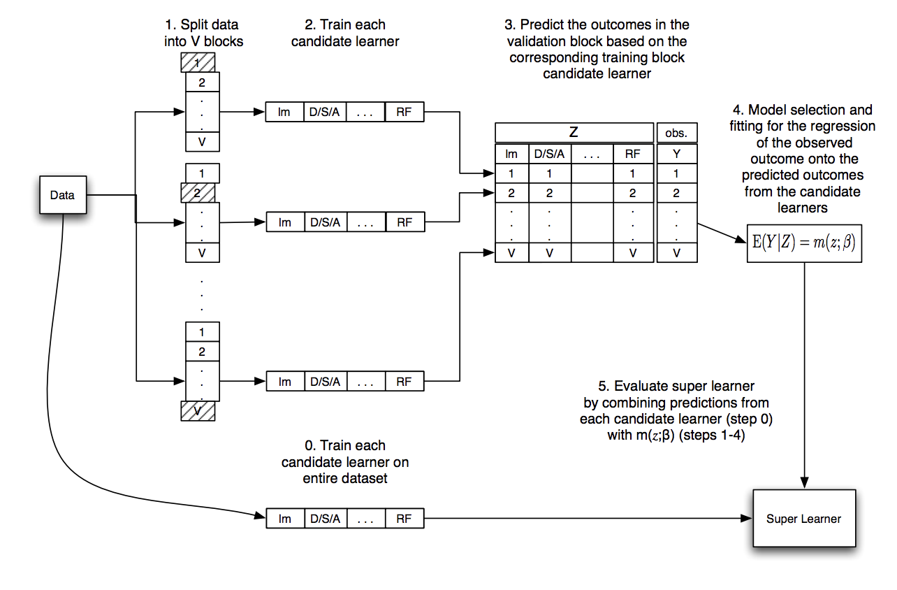
Another visual guide for superlearning
The steps of the superlearner algorithm are summarized nicely in this graphic in Chapter 3 of the Targeted Learning book:
Acknowledgments
Thank you to Eric Polley, Iván Díaz, Nick Williams, Anjile An, and Adam Peterson for very helpful content (and design!) suggestions for this post.
References
MJ Van der Laan, EC Polley, AE Hubbard, Super Learner, Statistical applications in genetics and molecular, 2007
Polley, Eric. “Chapter 3: Superlearning.” Targeted Learning: Causal Inference for Observational and Experimental Data, by M. J. van der. Laan and Sherri Rose, Springer, 2011.
Polley E, LeDell E, Kennedy C, van der Laan M. Super Learner: Super Learner Prediction. 2016 URL https://CRAN.R-project.org/package=SuperLearner. R package version 2.0-22.
Naimi AI, Balzer LB. Stacked generalization: an introduction to super learning. Eur J Epidemiol. 2018;33(5):459-464. doi:10.1007/s10654-018-0390-z
LeDell, E. (2015). Scalable Ensemble Learning and Computationally Efficient Variance Estimation. UC Berkeley. ProQuest ID: LeDell_berkeley_0028E_15235. Merritt ID: ark:/13030/m5wt1xp7. Retrieved from https://escholarship.org/uc/item/3kb142r2
M. Petersen and L. Balzer. Introduction to Causal Inference. UC Berkeley, August 2014. www.ucbbiostat.com
Session Info
sessionInfo()R version 4.1.2 (2021-11-01)
Platform: x86_64-apple-darwin17.0 (64-bit)
Running under: macOS Big Sur 10.16
Matrix products: default
BLAS: /Library/Frameworks/R.framework/Versions/4.1/Resources/lib/libRblas.0.dylib
LAPACK: /Library/Frameworks/R.framework/Versions/4.1/Resources/lib/libRlapack.dylib
locale:
[1] en_US.UTF-8/en_US.UTF-8/en_US.UTF-8/C/en_US.UTF-8/en_US.UTF-8
attached base packages:
[1] splines stats graphics grDevices utils datasets methods
[8] base
other attached packages:
[1] SuperLearner_2.0-28 gam_1.22-2 foreach_1.5.2
[4] nnls_1.4 gt_0.9.0 forcats_0.5.1
[7] stringr_1.5.0 dplyr_1.1.2 purrr_0.3.5
[10] readr_2.1.2 tidyr_1.2.1 tibble_3.2.1
[13] ggplot2_3.4.0 tidyverse_1.3.2
loaded via a namespace (and not attached):
[1] httr_1.4.2 sass_0.4.5 jsonlite_1.8.4
[4] modelr_0.1.8 Formula_1.2-4 assertthat_0.2.1
[7] googlesheets4_1.0.0 cellranger_1.1.0 yaml_2.3.7
[10] pillar_1.9.0 backports_1.4.1 lattice_0.20-45
[13] glue_1.6.2 digest_0.6.31 rvest_1.0.2
[16] colorspace_2.0-3 htmltools_0.5.4 Matrix_1.3-4
[19] pkgconfig_2.0.3 broom_1.0.1 earth_5.3.1
[22] haven_2.4.3 scales_1.2.1 ranger_0.14.1
[25] TeachingDemos_2.12 tzdb_0.2.0 googledrive_2.0.0
[28] farver_2.1.1 generics_0.1.3 ellipsis_0.3.2
[31] withr_2.5.0 cli_3.6.1 survival_3.2-13
[34] magrittr_2.0.3 crayon_1.5.0 readxl_1.3.1
[37] evaluate_0.20 fs_1.6.2 fansi_1.0.3
[40] xml2_1.3.3 tools_4.1.2 hms_1.1.1
[43] gargle_1.2.0 lifecycle_1.0.3 munsell_0.5.0
[46] reprex_2.0.1 glmnet_4.1-3 plotrix_3.8-2
[49] compiler_4.1.2 rlang_1.1.1 plotmo_3.6.1
[52] grid_4.1.2 iterators_1.0.14 rstudioapi_0.13
[55] htmlwidgets_1.6.2 labeling_0.4.2 rmarkdown_2.20
[58] gtable_0.3.1 codetools_0.2-18 DBI_1.1.2
[61] R6_2.5.1 lubridate_1.8.0 knitr_1.42
[64] fastmap_1.1.0 utf8_1.2.2 shape_1.4.6
[67] stringi_1.7.12 Rcpp_1.0.10 vctrs_0.6.2
[70] dbplyr_2.1.1 tidyselect_1.2.0 xfun_0.39